

You own memory stocks because AI usage is growing. Then a new model promises to use less memory. Does that undermine the investment case, or make more AI applications affordable?
KV cache helps turn that argument into questions you can actually test. The important variables are not just model size. They include how much context is retained, how many requests are active together, and where that context is stored.
Sources checked October 24, 2026. Numerical scenarios are original illustrations, not measurements of a named model or investment recommendations.
What is KV cache in AI inference?
During autoregressive generation, a Transformer can retain keys and values computed for earlier tokens and reuse them while producing later tokens. That retained intermediate state is the key-value, or KV, cache. A token is a unit processed by the model, not necessarily a word. Hugging Face documents the basic mechanism.
Think about a user who uploads a long report and asks several follow-up questions. Reusing relevant computation can avoid processing the same context from scratch. Whether the cache survives between requests, and for how long, depends on the serving implementation.
Model weights, conversation history and KV state are different
Weights are the model’s learned numerical parameters. Conversation history is the input and output content. KV state is an intermediate representation produced while processing that content. A conversation remaining on your screen does not prove its cache remains resident on a GPU.
This distinction matters for investors. A model’s weight size does not establish how many long conversations one accelerator can serve. Nor should every historical conversation be assumed to occupy accelerator memory forever. Both shortcuts can produce a very large, very misleading demand estimate.
How to calculate KV cache memory: a worked example
For a simple layout that stores uncompressed keys and values of equal shape at every layer, theoretical capacity follows this relationship:
The leading 2 counts keys and values. If sessions have different context lengths, sum their retained tokens instead of assuming every session is full.
Assume an imaginary configuration with 80 layers, eight KV heads, a head dimension of 128 and two bytes per element. Each cached token requires 327,680 bytes, or 320 KiB. A session retaining 131,072 tokens therefore requires 40 GiB of theoretical KV storage. Eight such sessions require 320 GiB.
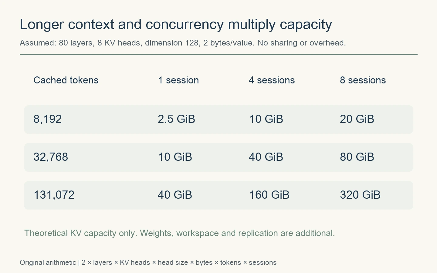
Why GB, GiB and “128K” need a definition
Here, 128K means 131,072 tokens. Substituting 128,000 gives approximately 39.06 GiB. And 40 GiB is about 42.95 decimal GB. These differences become material when multiplied across large fleets.
The formula does not include model weights, activation workspace, reserved capacity, cache-block management, replication or device placement. It is a starting point for an explicit scenario, not a specification for buying hardware. Parameter count alone cannot supply all the inputs. The model and implementation must reveal the relevant dimensions.
GQA, quantization and reuse can reduce the footprint
Use KV heads, not query heads, in the equation
Grouped-query attention lets multiple query heads share keys and values. A configuration with 64 query heads and eight KV heads uses eight for that term in the cache equation. Substituting 64 overstates this component eightfold. The original GQA paper describes the shared-head design.
Lower-precision cache storage can reduce bytes per element. But “four-bit weights” does not mean “four-bit KV.” Read what has actually been quantized, and consider quality, latency and hardware support separately.
Compressed and windowed architectures need their own calculation
The DeepSeek-V2 paper describes multi-head latent attention, or MLA, which uses a compressed representation. Sliding-window and hybrid attention also change what is retained. Applying a full-context, identical-layer formula without adjustment can misstate their footprint.
Shared prefixes can change concurrency arithmetic too. If compatible requests reuse cached blocks, multiplying complete context length by every user can overcount. TensorRT-LLM documents cross-request block reuse. It is conditional reuse, not permission to assume that all users’ private conversations share one cache.
For an investor, the useful habit is to identify the technology that changes each coefficient. Is the model retaining fewer bytes? Fewer tokens? More shared prefixes? Or moving data between tiers? Those mechanisms have different implications for physical memory and system performance.
Advertisement
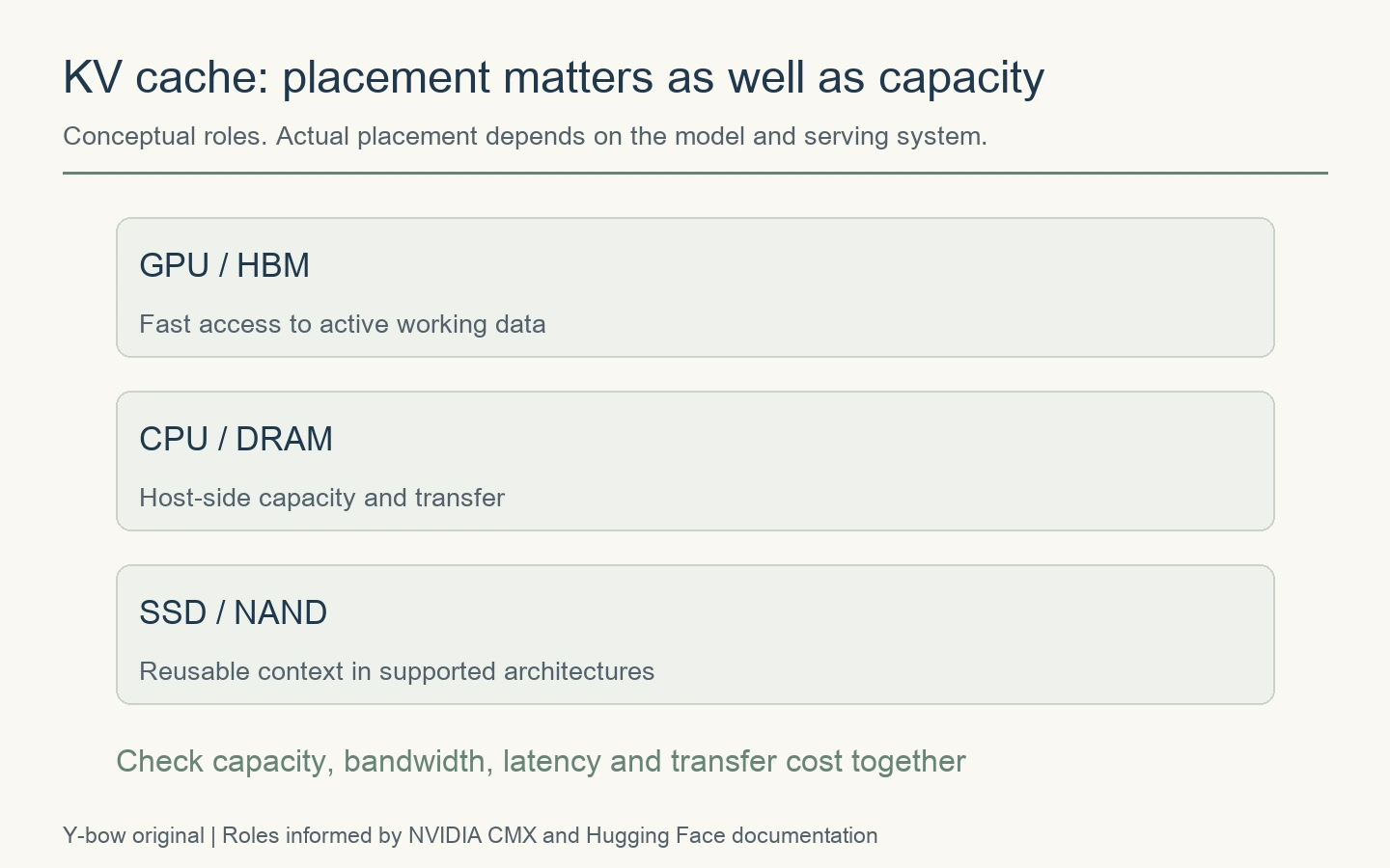
HBM vs DRAM vs SSD: where does inference context live?
← Swipe to view the full table →
| Location | Potential role | Constraint to check |
|---|---|---|
| GPU HBM | Fast access to active working data | Capacity, bandwidth, power and implementation |
| Host DRAM | Host-side capacity and transfers | CPU–GPU interconnect and transfer time |
| SSD / NAND | Context retention and reuse in supported tiers | Latency, throughput, endurance and orchestration |
Having somewhere to store the data does not mean it can be retrieved quickly enough to keep the accelerator busy. Capacity, bandwidth and latency are different measurements. Hugging Face’s cache-strategy documentation describes trade-offs such as moving cache state to the CPU. Saving device memory can come with additional transfer overhead.
CMX extends the hierarchy; it does not abolish HBM
NVIDIA describes CMX as a shared context tier powered by BlueField-4 that extends GPU memory. Its technical explanation links storage, networking and compute. That is a more specific claim than “SSDs replace HBM.” Vendor performance improvements also depend on workload and comparison conditions.
In its June 2, 2026 announcement, Kioxia distinguishes CM SSDs for KV-related storage, GP products for separate high-IOPS applications, and LC capacity-oriented storage. These are different jobs. The announcement describes products and strategy at that date; it is not evidence of realized October sales for each application.
Does more efficient AI reduce memory demand?
It can. It can also coexist with more total capacity. The direction depends on usage rather than on an efficiency headline alone.
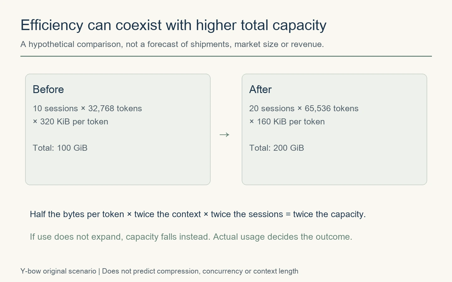
The illustration starts with ten concurrent sessions, 32,768 cached tokens each and 320 KiB per token: 100 GiB. Halving the bytes while doubling both session count and context gives 200 GiB. If usage stays unchanged instead, halving bytes reduces the requirement to 50 GiB.
Neither outcome is a law of AI economics. Some customers may use efficiency gains to lower the cost of an unchanged workload. Others may run longer investigations or more simultaneous agents. Budget limits, useful output quality and application design determine what happens next.
I would write the drivers separately: longer retained context, more simultaneous work, longer retention, then compression, reuse and eviction. It becomes much harder to turn every technology announcement into the same bullish—or bearish—conclusion.
Five checks before turning cache growth into a memory-stock thesis
← Swipe to view the full table →
| Step | Evidence to seek | Shortcut to avoid |
|---|---|---|
| 1 Usage | Retained context, concurrency and utilization | Treating registered users as simultaneous sessions |
| 2 Architecture | Which bytes reside in which tier | Allocating every byte to one supplier category |
| 3 Adoption | Qualification, shipment and deployment stages | Treating development as completed sales |
| 4 Revenue | Volume, pricing, mix and competition | Equating bit growth with dollar growth |
| 5 Cash | Margins, R&D, investment and collections | Assuming demand growth guarantees shareholder value |
An SSD gaining a new inference role is a technical development. A supplier earning durable returns from it also requires adoption, pricing power and disciplined costs. Capacity expansion can be necessary while still leaving weak free cash flow.
For company roles, see the HBM, DRAM and NAND industry map. For the conditions under which demand might change cyclicality, see five tests for a durable AI memory supercycle. The calculation here helps define the physical requirement; those articles examine the businesses around it.
Related full-length video: Why GPUs Need HBM: Memory Bandwidth Explained by Reimu & Marisa, from our English-language channel. It provides a visual companion to the capacity-versus-bandwidth distinction.
KV cache questions investors often ask
Does twice the cache mean twice the HBM?
No fixed ratio follows. Placement, sharing, compression and scheduling can change. A system may also encounter bandwidth or transfer constraints before running out of nominal capacity.
Is RAG storage the same thing as KV cache?
No. Retrieval-augmented generation brings external information into a model’s input. Processing that input can create KV state, but the external document store and the inference cache are distinct. Do not count one as the other.
Can this equation forecast the memory market?
Not on its own. It lacks actual deployment volumes, usage, refresh cycles, tier placement and prices. A useful investment model records what is unknown and identifies the observations that would change the thesis.
Sources, assumptions and updates
Primary references are linked beside the relevant claims: Hugging Face documentation, the GQA and DeepSeek-V2 papers, NVIDIA CMX and TensorRT-LLM, and Kioxia’s dated announcement. The three diagrams and comparison tables are original. No source chart has been reproduced.
The worked equation assumes uncompressed equal-shaped keys and values, no shared cache and the stated concurrent sessions. It excludes weights, workspace, reservations and replication. Product claims and realized shipments should be refreshed separately as companies update their disclosures. Announcing a new role is not the same event as earning revenue from it.








Comments